Charts are a powerful and easy-to-use tool in Google Sheets that can help you quickly visualize your data, making it easier to understand and analyze. With various chart types available, such as line, bar, column, pie, and scatter charts, you can easily create visual representations of your data to help you better understand trends and relationships within your data set.
Whether you are working with large or small data sets, charts in Google Sheets are designed to be intuitive and user-friendly. You can easily customize the look and feel of your charts by adjusting various settings, such as color schemes, labels, and axes. Additionally, you can interact with your charts in real-time by adding filtering or sorting options to make exploring and understanding your data more accessible.
If you are looking for a simple and effective way to visualize and analyze your data using Google Sheets, then take advantage of the powerful charting capabilities available on this platform. With its easy-to-use interface and wide range of customization options, you can quickly create engaging visualizations that will help you gain valuable insights into your data.


How do you add the x-axis to Google Sheets?
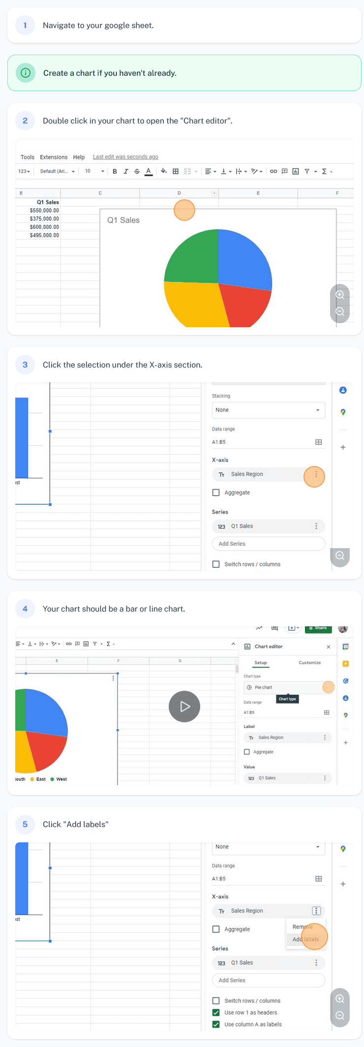
- Open a new Google sheet in your Google Drive and click on the “Add-ons” tab at the top of your screen.
- Select the “Chart” option in the dropdown menu, which will open a new window with various chart types.
- Select the “X-Axis” option, which will open a dialog box where you can customize your X-axis settings.
- Enter any values you want to appear along the x-axis, such as periods or numerical values, and then tweak other settings to get your desired chart format.
- When you are finished making changes, click the “Save” button at the bottom of the dialog box, then review your chart to ensure everything looks correct. If needed, you can make further adjustments by clicking on individual elements within your chart and editing them directly.
- Once you are happy with your chart, click the “Publish” button in the upper right corner of your screen to save it to your Google Drive and share it with others as needed. You can embed your chart directly into an online document or website for quick access or sharing.
If you want screenshots like this and step-by-step guides for any process, try the free Scribe .
.
Let us summarize the screenshots above:
The first step in adding an x-axis in Google Sheets is to open a new spreadsheet in your Google Drive account. Once you have unlocked your spreadsheet, click on the “Add-ons” tab at the top of the page and click “Script Gallery.”
Next, you must search for the script “GM Chart X-Axis,” a handy tool for quickly adding an x-axis to any chart or graph in your spreadsheet. Click on the “Install” button next to this script to automatically add it to your spreadsheet.
Once you have installed the GM Chart X-Axis script, you only need to select any chart or graph on your sheet and click on the “Draw X-Axis” option from the dropdown that appears. This will add an x-axis that extends across your entire chart, giving you more control over how your data is displayed.
To fine-tune your x-axis further, several additional options can be customized using the tools provided by this script. For example, you can change the scale, set where zero is located along the x-axis, and add labels and other formatting options to customize your chart further.
Adding an x-axis in Google Sheets is a relatively simple process requiring only a few basic steps. With these easy instructions, anyone can learn how to add an x-axis and get more out of their data visualization tools in Google Sheets.

Learn more about authors in Nimblefreelancer's team biography page.
- 6 Proven Ways SaaS Founders Actually Get Customers (With Real Examples) - December 17, 2025
- Facebook Ads to Get Followers! - December 27, 2024
- ClickUp vs. Slack - December 20, 2024