Legend is a term used to describe the graphical representation of data in charts and graphs. In a typical legend, each graphic element on the chart or graph represents a data series or an individual data point. Some legends also include information about the data type defined, such as the specific units used.
Using legends in charts can help make complex data more accessible to understand and interpret. For example, when dealing with large amounts of data across multiple periods or geographic regions, tracking how all the different lines, colors, and symbols correspond to specific pieces of information can be difficult. By including a legend that clearly labels each element on the chart, it becomes much easier to follow trends in the data and make informed decisions based on that information.


Many charts and graphs can include a legend, including line graphs, bar graphs, scatterplots, pie charts, and more. Whether using these tools for business analysis, scientific research, or another purpose, it is essential to consider how best to present your data so that it is easy for others to understand and interpret. With careful attention to detail in your legend design and layout, you can help ensure that your charts are as clear and compelling as possible.
How to Add a Legend to Your Chart in Google Sheets?
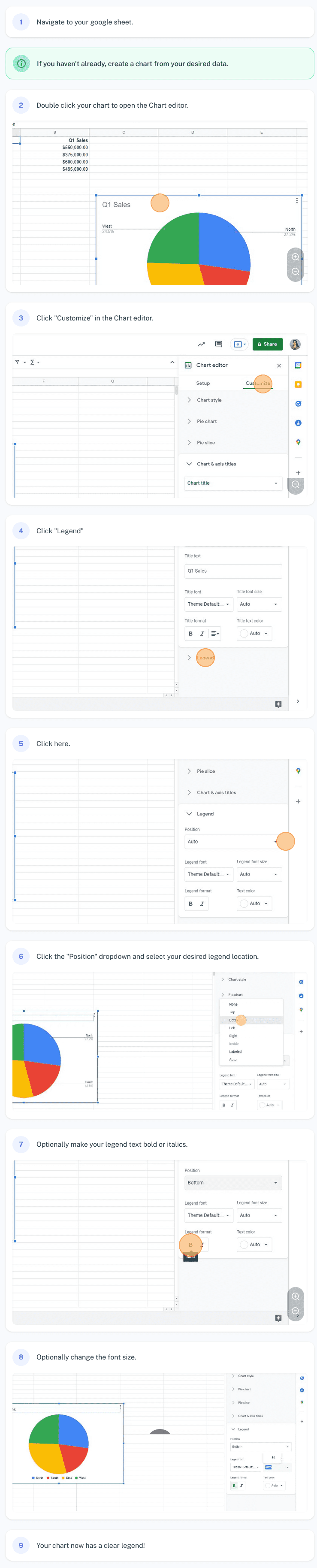
- Start by opening a new Google Sheets document and selecting the chart to which you want to add a legend.
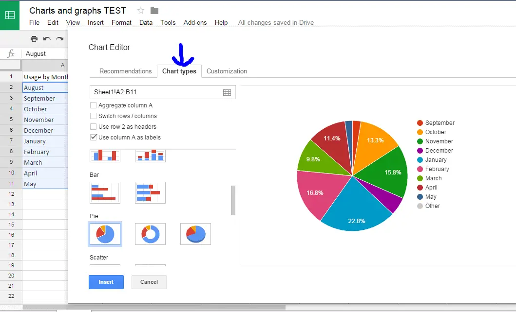
- Next, click on the “Format” tab at the top of your screen and select “Legend” from the drop-down menu.
- In the pop-up window that appears, customize the style and placement of your legend as needed. This window also allows you to display or hide labels for each data point in your chart.
- Once you have finished making any necessary changes, click “OK” to save your settings and add a legend to your chart.
- Finally, if you want to make further adjustments to your legend after it has been added, click and drag it around the chart or use the controls under the Format tab to change its size and appearance.
If you want screenshots like this and step-by-step guides for any process, try the free Scribe .
.
So let us summarize what you can see in the screenshots above:
One of the easiest ways to add a legend to your chart in Google Sheets is using the Data Labels feature. First, select your chart and navigate to the “Format” tab. Next, click on the “Data Labels” option in the sidebar, then choose your preferred label placement (either above or below each data point).
To customize your chart legend further, you can adjust the font size, color, and alignment. Additionally, you may want to add some additional formatting elements, such as titles or background colors, to make your chart stand out even more.
Regardless of which approach you take when adding a legend to your Google Sheets chart, it is essential to remember that charts are an excellent tool for visualizing data and presenting your findings in an easy-to-understand format. So whether creating charts for business or fun, take full advantage of all the tools and features in Google Sheets!

Learn more about authors in Nimblefreelancer's team biography page.
- 6 Proven Ways SaaS Founders Actually Get Customers (With Real Examples) - December 17, 2025
- Facebook Ads to Get Followers! - December 27, 2024
- ClickUp vs. Slack - December 20, 2024